Handwritten Notes on Flash Attention

Attention is not slow because of the math. Multiplying $Q K^\top$ and then multiplying by $V$ is a perfectly reasonable number of FLOPs for a modern GPU. It’s slow because the $N \times N$ score matrix has to be written to HBM, read back for the softmax, written again, and read one more time for the multiply by $V$. The GPU spends most of the wall clock waiting on memory while the tensor cores sit around doing nothing.

Flash Attention’s fix is to never materialize that matrix. It walks over blocks of $Q$, $K$, $V$ that fit in on-chip SRAM, and keeps a running softmax so it can produce the exact same output without ever holding a full row of scores in memory. Not an approximation — the same numbers, computed in a smarter order.

These are my handwritten notes working through the paper. The whole PDF is embedded below, and the rest of the post walks through it page by page.

The short version

Three moving parts, and the notes hit them in order. Page 2 shows that softmax can be computed incrementally, then annotates Algorithm 1 and the SRAM budget that decides the block sizes. Page 3 grinds through the one line of the algorithm that looks like a hack — the output rescaling — and shows it isn’t. Page 4 counts the memory traffic and gets $O(N^2 d^2 M^{-1})$ HBM accesses instead of $\Theta(N^2)$.

Page 2 — A softmax that never sees the whole row

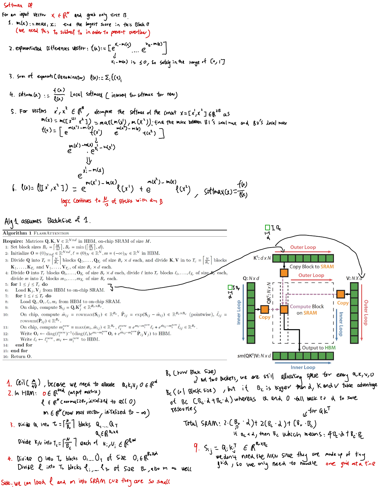
The obstacle to tiling attention is softmax. It needs a maximum over the whole row (for numerical stability) and a sum over the whole row (for the denominator), which is an inconvenient thing to need when you are deliberately looking at one block at a time. The top of this page fixes that by defining softmax through three running statistics instead of one pass.

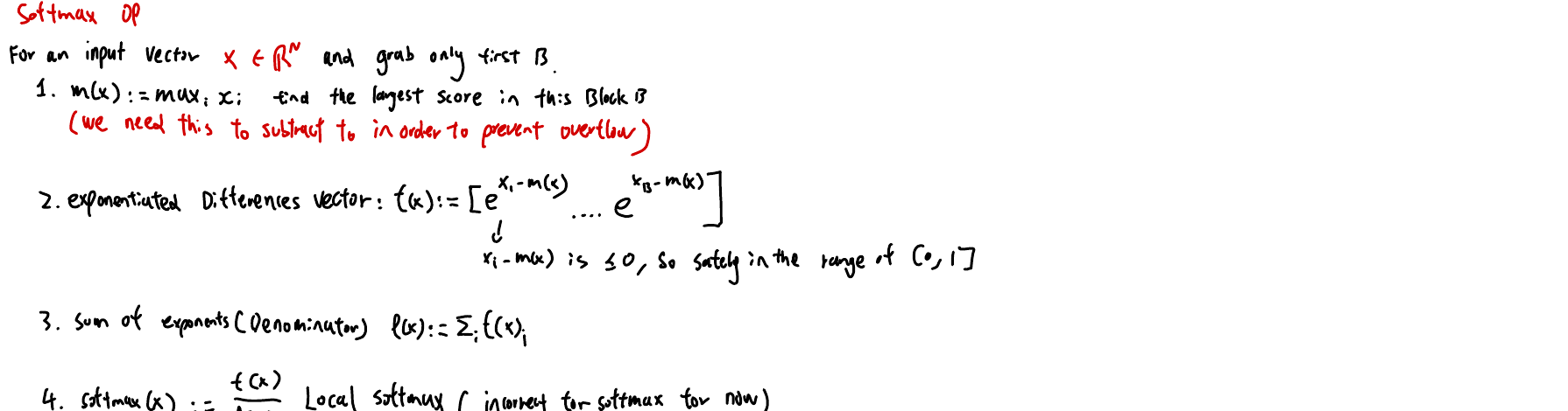
For an input vector $x \in \mathbb{R}^N$, grab only the first block of size $B$:

The subtraction in step 2 is the standard overflow guard. Every exponent $x_i - m(x)$ is $\leq 0$, so every entry of $f(x)$ lands safely in $(0, 1]$ and nothing blows up. It also means $m$ is baked into $f$ and $\ell$, which is exactly the problem: a block computed against its own local max is, as the note bluntly puts it, “incorrect for softmax for now.”

Merging two blocks

Steps 5 and 6 are where it becomes an algorithm. Take two blocks $x^{1}, x^{2} \in \mathbb{R}^{B}$ and concatenate them into $x = [\,x^{1}, x^{2}\,] \in \mathbb{R}^{2B}$. The new max is free:

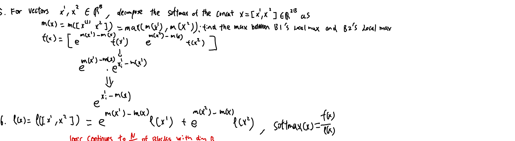
The exponent vectors need a correction, and it’s a single scalar per block. Whatever a block computed against its own local max gets re-based to the global one:

The whole trick is one line of exponent arithmetic, drawn in the notes with a big $\Downarrow$:

The local max cancels itself out. Sum both rescaled halves and you get the denominator, which is step 6:

And since the merge takes two blocks and returns something with the same shape as a block, you can just keep going — “logic continues to $N/B$ blocks with dim $B$.” Carry $(m, \ell)$ as state, fold in one block at a time, and the exact softmax falls out at the end. Two scalars per row is the entire price.

Algorithm 1, annotated

The middle of the page is the algorithm box from the paper, with a reminder in the margin that it assumes a batch size of 1 — real implementations add batch and head dimensions on top, which changes nothing conceptually and everything about the indexing.

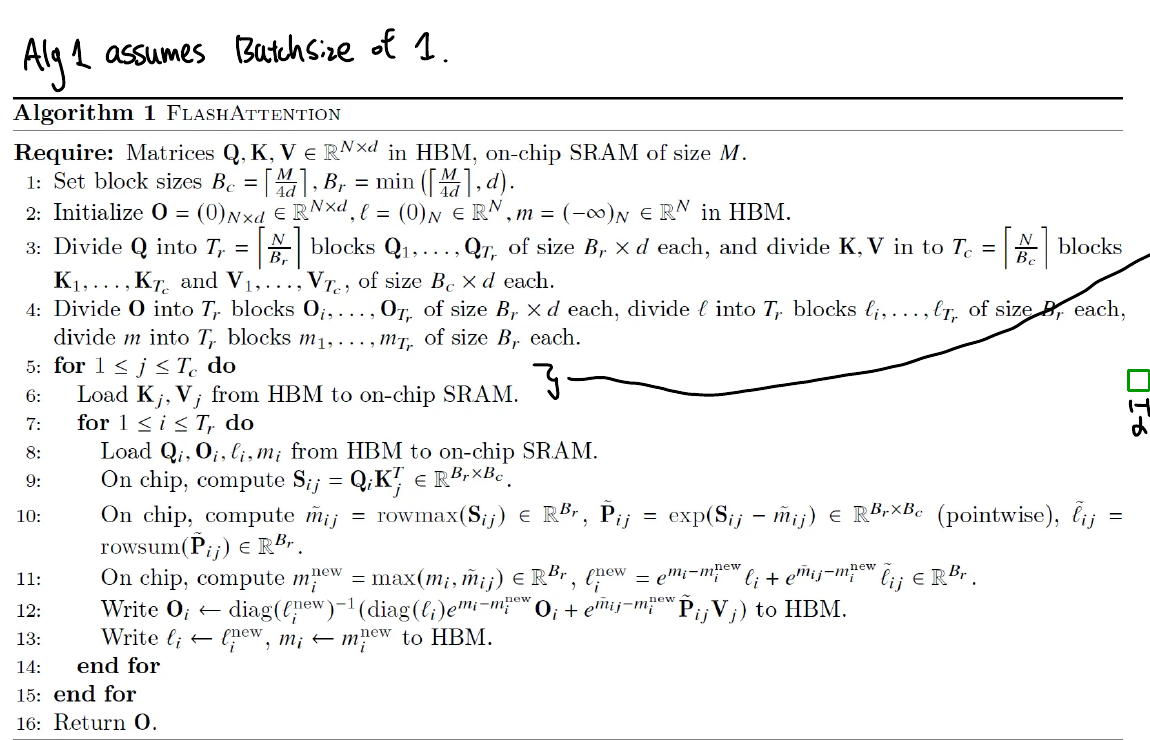
Line 1 picks the block sizes from the SRAM capacity $M$, and this is the line worth staring at:

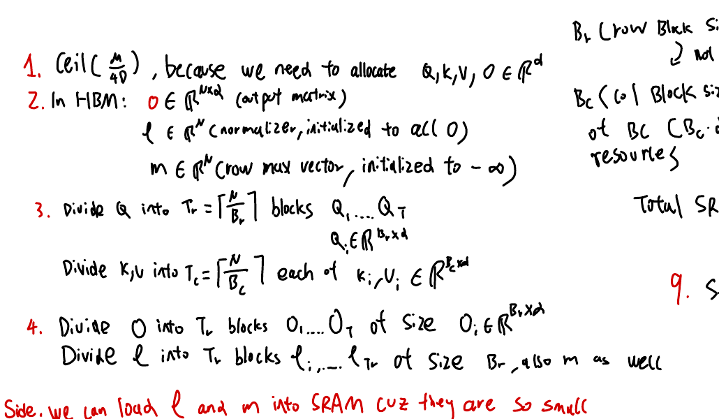
The $4d$ is there because a block of rows costs four $d$-wide tiles at once: you are holding $Q$, $K$, $V$ and $O$ simultaneously. Divide the budget four ways and that’s how many rows fit.

Line 2 sets up what stays in HBM:

• •$O \in \mathbb{R}^{N \times d}$ — the output matrix, initialized to zero.
• •$\ell \in \mathbb{R}^{N}$ — the running normalizer, initialized to all 0.
• •$m \in \mathbb{R}^{N}$ — the running row-max vector, initialized to −∞ (so the first real max always wins).

Lines 3 and 4 do the tiling. $Q$ splits into $T_r = \lceil N/B_r \rceil$ blocks of shape $B_r \times d$; $K$ and $V$ each split into $T_c = \lceil N/B_c \rceil$ blocks of shape $B_c \times d$. $O$ follows $Q$’s partition, and so do $\ell$ and $m$ — which, being $B_r$-length vectors rather than matrices, are small enough to keep resident in SRAM without anyone noticing.

Who loops over what

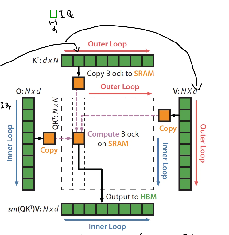
The outer loop (line 5) walks over the $K$, $V$ blocks; the inner loop (line 7) walks over the $Q$ blocks. So a single $K_j, V_j$ pair is loaded into SRAM once and reused against every query block, while $Q_i, O_i, \ell_i, m_i$ get cycled through underneath it. Every block that gets computed on-chip is written back to HBM as a $B_r \times d$ slice of the output — never as part of an $N \times N$ anything.

Line 9 is where that pays off. The score block is $S_{ij} = Q_i K_j^\top \in \mathbb{R}^{B_r \times B_c}$, and as the note in the corner says: we don’t need the $N \times N$, since it’s made of these tiny grids and we only ever handle one grid at a time.

The SRAM budget

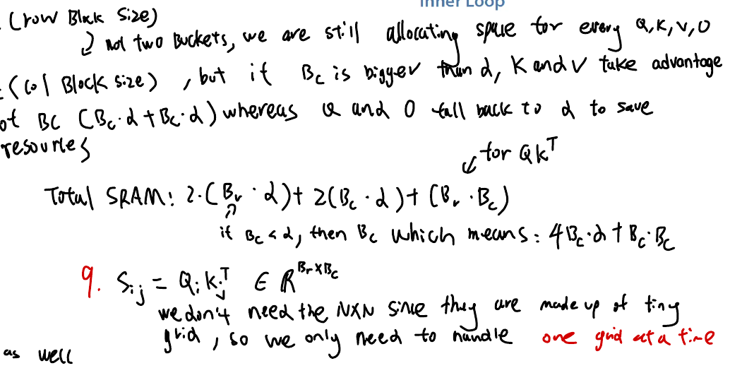
Adding up what a single iteration needs resident on-chip:

The asymmetry between $B_r$ and $B_c$ is deliberate. $K$ and $V$ get the full column block size, because a wider $B_c$ means more reuse per load. But $Q$ and $O$ are capped at $d$ rows — they fall back to $d$ to save resources, since making them taller buys nothing and costs SRAM. When $B_c \leq d$ the min collapses and $B_r = B_c$, which tidies the budget to:

Page 3 — Why line 12 isn’t a hack

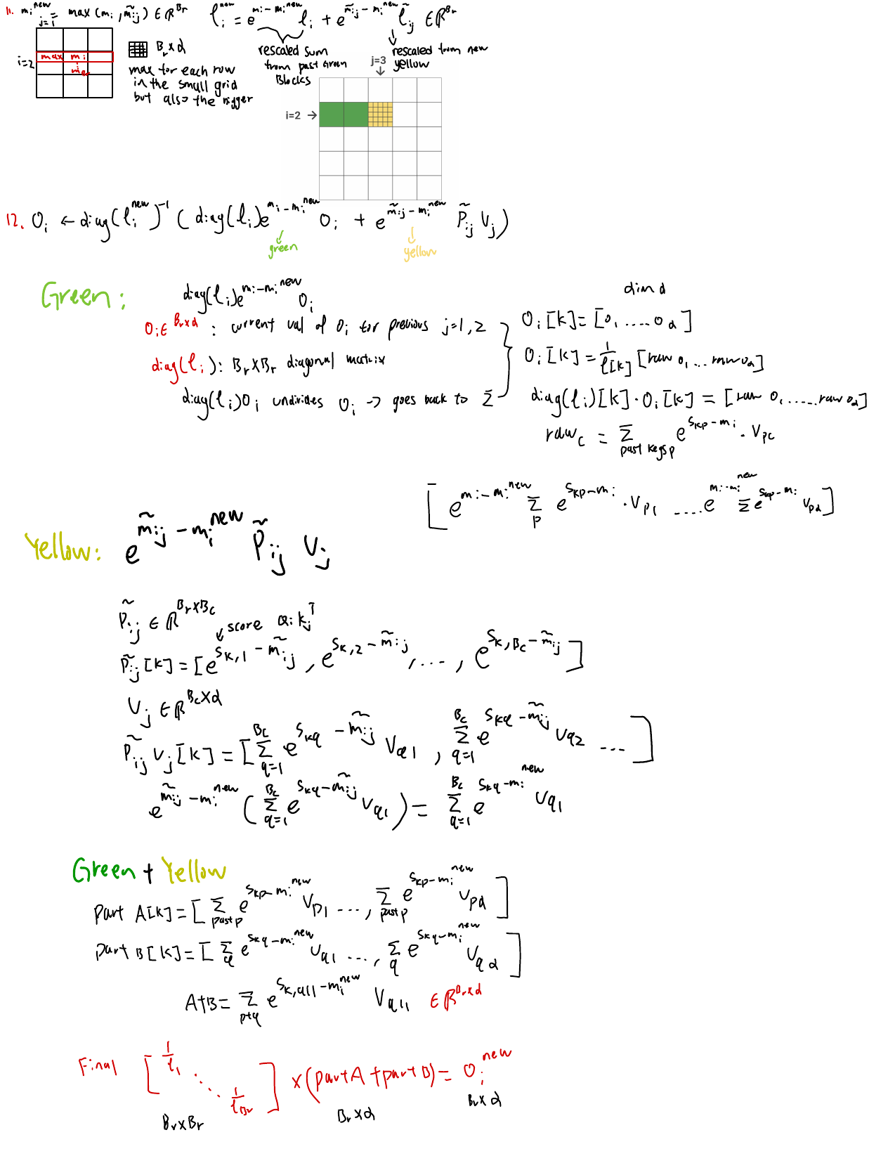
Line 12 is the line that makes people squint. It rescales the output block you already computed by a ratio of exponentials and a pair of diagonal matrices, and it is not at all obvious that what comes out the other side is a correct softmax-weighted average. This whole page is the check.

First, the running statistics

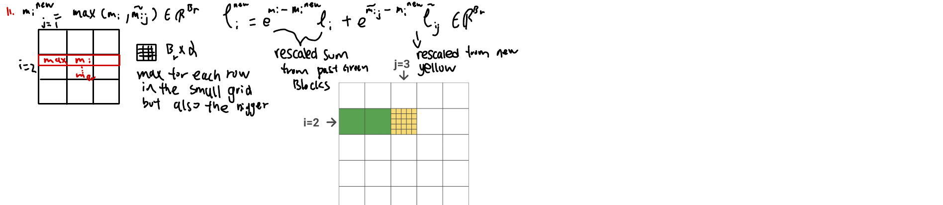
Line 11 updates the two per-row statistics. The new max is the running max against the current block’s max:

The two grids in the margin are the whole mental model. The small one makes the point that the max is taken per row of the block, not over the block as a whole — row $i$ of the tile carries its own $m_i$, and that row-local max is simultaneously the running max for that row of the full attention matrix. The bigger grid colors row $i=2$: green for the key blocks $j = 1, 2$ already folded in, yellow for $j = 3$, the one currently on-chip. That color coding runs through the rest of the page.

The line itself

Read it as three moves: undo the old normalization, put both halves on a common exponent base, then re-normalize with the new denominator. The rest of the page checks the green and yellow terms separately.

Green: rewinding the old output

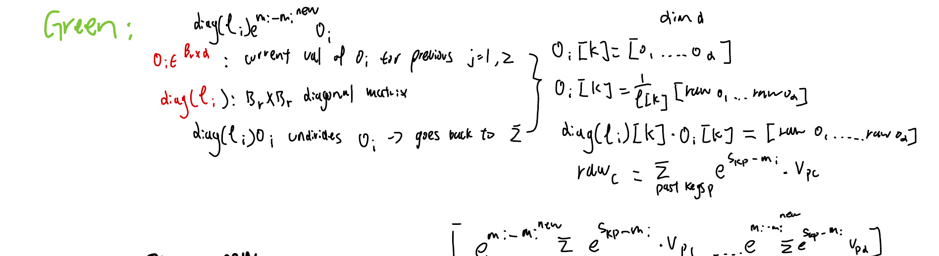
$O_i \in \mathbb{R}^{B_r \times d}$ is the current output for key blocks $j = 1, 2$ — a finished softmax average over the keys seen so far, meaning it has already been divided by $\ell_i$. Row $k$ of it is:

Multiplying by the diagonal matrix $\mathrm{diag}(\ell_i) \in \mathbb{R}^{B_r \times B_r}$ undivides it — each row is scaled by its own normalizer, which puts you back at the raw weighted sum:

That sum is still expressed relative to the old max $m_i$. One scalar multiply fixes it, using the same cancellation from page 2:

So the green term is the accumulated numerator over all past keys, rewritten in the new exponent base. No information lost, nothing approximated.

Yellow: the block in hand

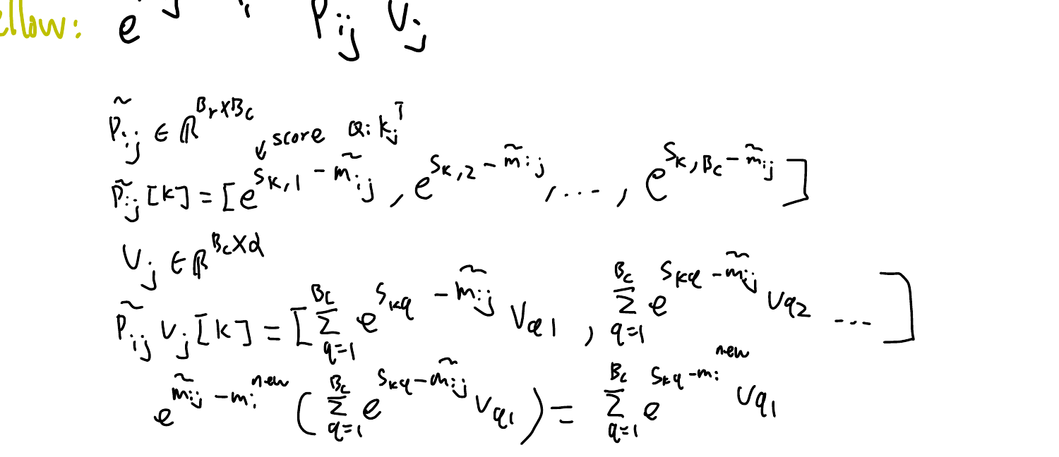
$\tilde P_{ij} \in \mathbb{R}^{B_r \times B_c}$ holds the exponentiated scores for the current tile, each entry taken against the tile’s local max $\tilde m_{ij}$:

Multiplying by $V_j \in \mathbb{R}^{B_c \times d}$ contracts over the $B_c$ keys in the tile, giving a $d$-dimensional row:

Then the same one-scalar re-basing as before:

Green + yellow

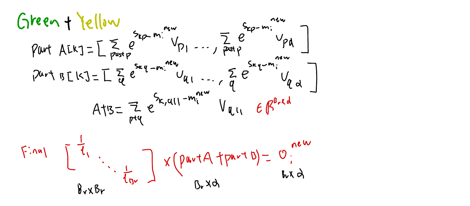
Both terms are now sums of $e^{\,s - m_i^{\mathrm{new}}} V$ over disjoint sets of keys, in the same exponent base. Which means they simply add:

That is exactly the numerator of a softmax taken over every key seen so far. Divide by the new normalizer — the $B_r \times B_r$ diagonal on the left — and you have the updated output block:

Which is the punchline of the page: $O_i$ is correct after every iteration, not just the last one. It’s always the exact attention output restricted to the keys processed so far, which is why the loop can stop caring about everything it has already thrown away.

Page 4 — Counting the memory traffic

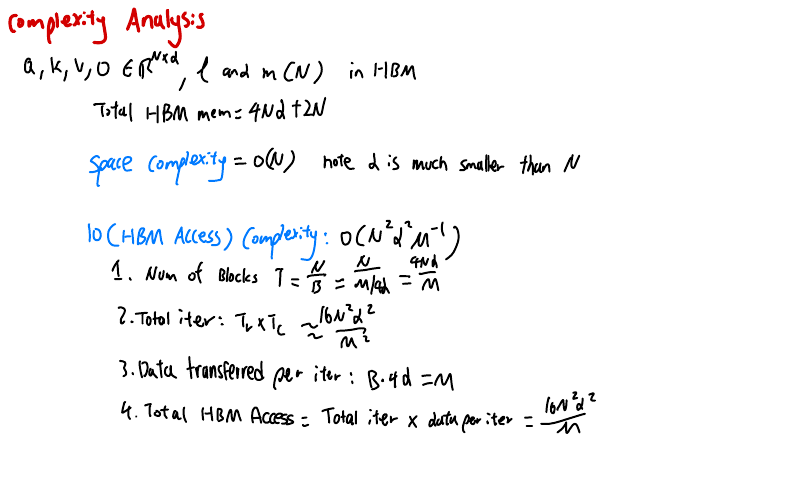
Start with what actually lives in HBM: $Q, K, V, O \in \mathbb{R}^{N \times d}$ plus the two vectors $\ell$ and $m$ of length $N$:

Treating the head dimension $d$ as a constant (it’s typically 64 or 128, while $N$ runs into the thousands), that is linear in sequence length. Standard attention has an $N \times N$ matrix sitting in there, so this is already the headline win.

Then the IO count, in four steps:

• •$T = \frac{N}{B} = \frac{N}{M/4d} = \frac{4Nd}{M}$ — number of blocks along one axis, since the block size comes from the SRAM budget.
• •$T_r \times T_c \approx \frac{16 N^2 d^2}{M^2}$ — total iterations of the doubly-nested loop.
• •$B \cdot 4d = M$ — data moved per iteration — one iteration's worth of Q, K, V, O tiles, which is a full SRAM's worth by construction.
• •$\frac{16 N^2 d^2}{M^2} \cdot M = \frac{16 N^2 d^2}{M}$ — iterations times bytes per iteration.

Compare that to standard attention’s $\Theta(Nd + N^2)$. The ratio is roughly $d^2 / M$, and on real hardware $M$ is on the order of 100 KB while $d^2$ is a few thousand — so the traffic drops by something like an order of magnitude. Note the direction of the $M$: bigger SRAM means fewer memory accesses, because bigger blocks mean more reuse per load. This is the rare complexity result where the constant factor of your hardware shows up in the exponent’s neighborhood and you’re glad about it.

What I took away

The thing worth remembering isn’t the algebra, it’s the framing. Flash Attention doesn’t reduce the number of operations at all — it does more arithmetic than standard attention, since every block re-scales work that was already done. It wins anyway, because on a modern GPU the arithmetic is nearly free and the memory movement isn’t.

The softmax decomposition on page 2 is what makes that trade legal. Everything after it is bookkeeping: carry $(m, \ell)$, re-base when the max moves, divide at the end. Once you’ve seen it, the same running-statistics pattern shows up everywhere — Welford’s algorithm for variance, streaming log-sum-exp, half of what a distributed reduce does.